Spy Journal 3.0 Filtering the web for you

When I wrote the how to use VLOOKUP and HLOOKUP article a few weeks ago I hinted at writing how to use the COLUMN, ROW, MATCH, INDEX and OFFSET functions to enhance the use of the VLOOKUP and HLOOKUP functions. Today we will look at the use of MATCH.

First of all here is a common scenario.

You create a table of say 4 columns, and then in another sheet you create a VLOOKUP function that returns results from the 4th column. EG =VLOOKUP(lookup_value,table_range,4,FALSE) where the 4 relates to the 4th column. This works great until one day you (or your colleagues) delete the 3rd column in the table, or insert another column in the middle of the table. Now your VLOOKUP fails as the 4th column either doesn’t exist, or is now actually the 5th column. In this case the VLOOKUP formula you created is just not flexible enough to handle the changes.

The following explanation builds on the dynamic range name process defined in my article written back in 2004. You will need to create a dynamic range name (in this example called table_header) that works on the header row of the table you are performing the VLOOKUP on.

In Excel 2007 Use the Name Manager from the Formula tab. In Excel 2003 and earlier use Edit Insert Name Define. In both versions CTRL F3 is the keyboard short cut.

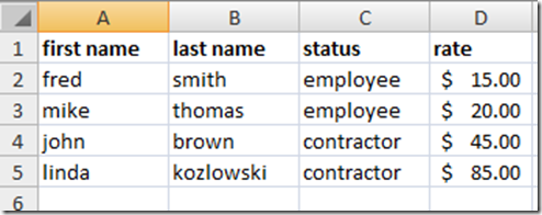
Here is my sample table of data in Sheet1.

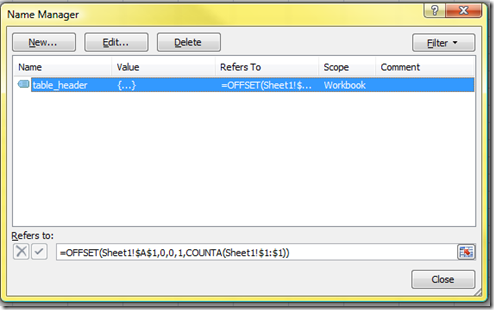
Create a new range name and in the reference enter the OFFSET formula for a row. (assuming table is built from column A out and there is no other data in the sheet)

=OFFSET(Sheet1!$A$1,0,0,1,COUNTA(Sheet1!$1:$1))

On another sheet  I have a VLOOKUP formula designed to return the pay rate of a selected employee from a drop down list.

Originally it was like the picture here with this formula =VLOOKUP(A2,Sheet1!A:D,4,FALSE)

Now in the VLOOKUP formula replace the column no (E.G. 4) with this MATCH formula MATCH(Sheet1!$D$1,table_header,0) so the total formula now reads like this =VLOOKUP(A2,Sheet1!A:D,MATCH(Sheet1!$D$1,table_header,0),FALSE)

What this does is tell the formula to use the value in the header row in the column you want and return its position in the table_header range. Even if you go and change the name of that column to something else it will still work. Inserting a column in the middle of the table, or deleting a column from the table will not stop the VLOOKUP function from performing correctly.

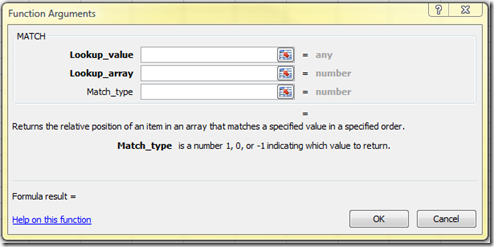
Finally, here is the Excel function layout and help for the MATCH function. Note the Match type argument can be –1, 0 or 1. Read the details below as to when you should use these values.

The MATCH function searches for a specified item in a range of cells, and then returns the relative position of that item in the range. For example, if the range A1:A3 contains the values 5, 25, and 38, then the formula

=MATCH(25,A1:A3,0)

returns the number 2, because 25 is the second item in the range.

Use MATCH instead of one of the LOOKUP functions when you need the position of an item in a range instead of the item itself. For example, you might use the MATCH function to provide a value for the row_num argument of the INDEX function.

Syntax

MATCH(lookup_value, lookup_array, [match_type])

The MATCH function syntax has the following arguments:

• lookup_value  Required. The value that you want to match in lookup_array. For example, when you look up someone's number in a telephone book, you are using the person's name as the lookup value, but the telephone number is the value you want.

  The lookup_value argument can be a value (number, text, or logical value) or a cell reference to a number, text, or logical value.

• lookup_array  Required. The range of cells being searched.
• match_type  Optional. The number -1, 0, or 1. The match_type argument specifies how Excel matches lookup_value with values in lookup_array. The default value for this argument is 1.

  The following table describes how the function finds values based on the setting of the match_type argument.

  Match_type Behavior

  1 or omitted - MATCH finds the largest value that is less than or equal to lookup_value. The values in the lookup_array argument must be placed in ascending order, for example: ...-2, -1, 0, 1, 2, ..., A-Z, FALSE, TRUE.

  0 - MATCH finds the first value that is exactly equal to lookup_value. The values in the lookup_array argument can be in any order.

  -1 - MATCH finds the smallest value that is greater than or equal to lookup_value. The values in the lookup_array argument must be placed in descending order, for example: TRUE, FALSE, Z-A, ...2, 1, 0, -1, -2, ..., and so on.