Conditional formatting in Excel 2007 - entire row colours
I had an interesting question about conditional formatting posed in the comments by Stephen.
In a new sheet, I am trying to make a whole row turn red, green or amber depending on the value of one cell in that row, so I can easily see which jobs we have won, lost or are pending. Any 'IF' conditional formula I write gets thrown out by Excel. What am I doing wrong?
I promised him an answer so here it is.
For this exercise I am making some assumptions.
- You are using Excel 2007 format Excel spreadsheet (.xlsx or .xlsm). These instructions will not work in detail for Excel 2003, though the concept is similar.
- That there are 3 conditions we are looking for. Of course Excel 2007 allows more than 3 conditions so you can add more if you need. (One of the improvements on Excel 2003 that only allowed 3 rules)
- That the entire row is needed to be coloured. If you need a smaller section than change the formulas accordingly.
- That the entire worksheet needs this formatting. If you need a smaller section than change the formulas accordingly.
- That the conditional formats are going to be based on a cell that returns a specific result based on some other rule.
The first thing I did was set up a spreadsheet using column H as my rule column. I often do something similar to this where I create a hidden column at the side of my data table and perform a IF function based calculation that returns me a value depending on the data evaluated. To use Stephens example I am assuming that jobs won have returned a 1, jobs pending returns a 0 and jobs lost a –1. These values can be anything – they are not relevant.
Now we are ready to create the conditional formatting rules.
The important thing to remember with conditional formatting when trying to work with more than just the selected cell is the absolute and relative cell selection rules. Read more about absolute and relative references if you need to.
Select the entire sheet (by clicking the gray triangle left of column A).
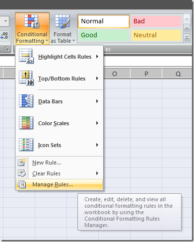
From the Home tab select the conditional formatting option and click Manage Rules.
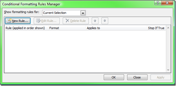
This brings up the Conditional Formatting Rules Manager.
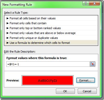
Select New Rule and then Use a formula to determine which cells to format.
Create a rule where the formula is =$H1=-1 and the format is a fill of red.
Click OK.
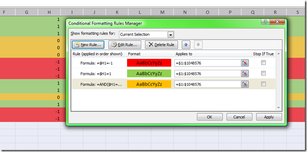
Now make a new rule where the formula is =$H1=1 and the format is a fill of green.
Lastly make a new rule where the formula is =AND($H1=0,$H1<>””) and the format is a fill of amber. This rule keeps the cells unfilled where there is nothing in column H.
Click Apply to view the result.
The trick here is that the cell reference $H1 allows the rule to be applied down to every row and use the value in column H for every cell in that row.
Columns could be formatted in the same manner using a rule value in a row by locking the row and allowing the column to alter. eg. H$1.
Feel free to comment if this was helpful, or if you have other questions that need solving.


Comments
Awesome! I had struggle with
Awesome!
I had struggle with this same question as well. I could manage it in Excel 2003 just fine (minus the limitations of 3 conditions), but couldn't for the life of me get this down...
Your instructions made it much more clear - (Jae smacks forehead and makes Homer "DOH!" after actually getting this to work!) - thanks so much!
-- Jae
glad to be of help Jae
glad to be of help Jae
I want to create IF function
I want to create IF function based on cells that are conditionally formatted.
Say, there are two criteria for supplier selection- Price and warranty. I have conditionally formatted them with 3 arrows (green, red and yellow). Now i want to score them as say Green = 4, red = 1 and yellow= 3. This score would have to be based on the display of the criteria cells (Price and warranty).
The table would be similar to below.
vendor Price Warranty Scores
A 10 2 6
B 9 2 6
C 4 2 7
A 6 2 7
B 7 2 6
C 8 1 4
A 9 1 4
B 12 2 6
A 15 3 7
B 18 2 4
Please mail me at: sukanto.ibs@gmail.com
I'm not an excel guru, far
I'm not an excel guru, far from one, but this post has really inspired me to go back and take a look at a lot of the spread sheets I have been making for my freelance web design accounting. This article can really help me improve accountability and potentially save a good amount of time and money doing so. The only question I have, would this work if I import a spread sheet into Google Docs?
Thanks, and again - great article!
Hi Shay no idea sorry - would
Hi Shay
no idea sorry - would love to hear what the result is. I havent done more than have a cursory look at google spreadsheets because they dont do what i need. they are a light weight spreadsheet in terms of their functionality. I dont know if they can even do any conditional formatting.
Can you try it and report back here?
Cheers
Tim
No it wouldn't sorry - Google
No it wouldn't sorry - Google docs is a very cut down basic spreadsheet system. Most of the advanced functionality we use and expect to see in the Office Excel application just isn't available in Google docs. the office live apps (which i have yet to test in full - may however. They are written by Office, but they also cut out some functionality. the fault isn't the app but rather the platform, converting to a web platform forces some platform based standards to be used rather than what can be done on your desktop application.
Thanks alot! It helps me to
Thanks alot!
It helps me to get an idea. I was thinking how to do that for 2 days. Thanks
Great! This helped.
Great! This helped.
It's hard to come by educated
It's hard to come by educated people in this particular subject, but you sound like you know what you're
talking about! Thanks
Hi there, i read your blog
Hi there, i read your blog from time to time and i own a similar one and i was just wondering if you get a lot of spam comments?
If so how do you stop it, any plugin or anything you can advise?
I get so much lately it's driving me mad so any assistance is very much appreciated.
we use mollom to trap spam
we use mollom to trap spam
What's up, I check your new
What's up, I check your new stuff daily. Your story-telling style is witty, keep up the good work!
I have numbers all below 1 ie
I have numbers all below 1 ie 0.001, 0.0123 and -0.001 etc. How can I conditional format a row using just negative or positive numbers as criteria please?
Hi John Just use the same
Hi John
Just use the same rules as above but use <0 and >0
Cheers
What if I want to use text to
What if I want to use text to determine my conditional formatting. For example I want to format all rows containg the word "YES", but when I use the formula you provided in your example above and I set to =YES it does nothing. If I replace the word YES with a number then it works fine.
Does this formula only work when formatting cells that contain numbers?
make sure you yse quotes
make sure you yse quotes around the text - i just did this one with the cells in column D
=$D1="YES"
That worked. Is that case
That worked. Is that case sensitive though? Because I thought I tried that yesterday...I typed "YES" in the formula, but I was typing yes in the actual cell and it wasn't working, but I could've had something else wrong.....either way it works now. THANKS
yes it is case sensitive -
yes it is case sensitive - glad to hear it works!
I tried this - but it colored
I tried this - but it colored my whole sheet the color of my first formula. I am using text (with "s) instead of numbers.
I am trying to color the rows that have been "Completed" with green, "Assigned" with orange, and "Backlog" with yellow. I followed your instructions, but after I type in the first formula, my whole sheet turns green. None of the other colors show. Please help - I am sooooo frustrated!! :/
email it to me and ill see
email it to me and ill see what you did wrong
I just had to thank you for
I just had to thank you for this...Spent a lot of time figuring it out and your article was like a light bulb
thanks
happy to be of help thanks
happy to be of help
thanks for the feedback
Cheers
Hi, This is similar to
Hi,
This is similar to something I am trying to accomplish, but not exactly, and I was wondering if you could help me out.
I'm trying to make a tracking sheet for workers who are required to review a certain case (columnA) every 3 months.
In columnB they enter the date they reviewed the case on that row. On the same row, I want the cell in columnC to be yellow if three months have elapsed since the date entered in columnB.
I'm sure this is possible, I just can't figure out how to do it.
Thanks!
sure is possible you need to
sure is possible
you need to understand how dates work in excel. they are all just a number
format the date cell as a number and see what i mean.
so if a date is a number then three months after that date will be the number +90
eg date+90 = 3 months after the date.
so if the date is less than today -90 then its is more than 3 months ago
= today()-90
by the way you could make the date cell in column B the coloured one - you don't have to go to column C
so in your conditional format in cell B1 use a formula like this
=TODAY()-90>B1
Note do not use the $ signs in the formula or it will not repeat correctly when you copy the format down.
hope this helps :)
I am looking at doing the
I am looking at doing the same sort of formatting, buti wouldlike for te entire row in which the cell with the formatting sits to change to the same color that I have created the formatting to do. I would also like it to flash as well. Any thoughts?
the whole row is
the whole row is easy
unfortunately i do not know of any ways to make the row flash
Fantastic, it worked!
Fantastic, it worked!
Thanks so much!
One more question: I removed
One more question:
I removed the dollar signs so that I could drag the formatting to other cells, but now when I sort the worksheet, the formatting doesn't follow :-(
If I add the dollar signs back, then the entire worksheet is formatted based on the the first cell :-(
How can I make the formatting follow the sort?
Thanks :-)
i just tested that exact
i just tested that exact example and it worked for me so maybe you are missing something
heres all the steps i just went through
entered dates in cells in column b - going back 1 year to current
selected cell b1 and added the conditional format by going to
- new rule
- use a formula to determine which cells to format
- adding =TODAY()-90>B1 as the rule
- selecting B1 and copying it
- selecting remainder of cells and pasting special formats
- sorting the column by values oldest to newest.
now if i select any cell and view the conditional format it has changed the range in which it appears but the formula is always =TODAY()-90>Bn where n is the row number of the cell
I hope there was something in there that helps you out
What happens when I do what
What happens when I do what you've suggested above is that I get basically 2 different conditional formatting rules. In the original cell from which I copied I have =TODAY()-90>B1 and in the Conditional Formatting Rules Manager under "applies to" it says "=$C$1."
In the rest of the cells the formula is "=TODAY()-90>B2" and in the rules manager under "applies to" it says "=$C$2:$C$12" which represents the cells to which I pasted the formatting. This doesn't change when I switch the sort order. C1 stays formatted the way it is, and the other cells stay formatted the way they are.
This poses a problem, because I want to be able to format cells for certain cases as "=Today()-90" and others as "=TODAY()-365". When I sort it I want the correct formatting to stay with the data. As I have it, the formatting stays where it is in the workbook regardless of the data.
Thanks for all your help!
rather than copying and
rather than copying and pasting to a specific range (which should include the copy cell anyway) you can edit the rule instead to say what range you want them to apply to - eg $C:$C
this will apply to the whole column and work no matter what cell it is in
the formula always says B1 but that is relative to the cell so works on the correct cell.
Of course if you apply it to the whole range you may want to add a rule or extend this rule to exclude cells that are blank
eg =AND(B1<>"",TODAY()-90>B1)
So I made that rule in cell C1 and applied it to $C:$C and it works when you sort it also.
See how you go.
But will that allow me to
But will that allow me to have some of the cells in column C as TODAY()-90>B1, and some as TODAY()-365>B1, and to have that formatting follow the sort?
Thanks!
no - not the way i wrote that
no - not the way i wrote that last answer
if you want two separate pieces of logic you would need to build that into the formula. think about how you would write an if statement that logically gave you the answer you need for the >90 and >365 values - this is what you would need to use.
a conditional format is just what it says it is - its a format based on a condition for a range. the condition needs to be a logical argument that can be solved as either true or false.
so you could write an argument that says if the date is more than 90 days ago then result or if the cell is more than 365 days than result
have a go and see if you can make it work in a single formula.
if not, you can write two separate formulas and have them both apply to the range $C:$C. excel will solve them in order. so you would want the 365 day one to be first i assume, and if a cell was not more than 365 days old it would look at the second rule and if it was more than 90 days old colour it.
let me know how you go
i'm trying to have 3 cells to
i'm trying to have 3 cells to turn to n/a from the input of another cell.
if i select yes from my cell in column H, 2 out of the three cells change to n/a and condtional format grey, however the middle cell has a drop down menu in this and wont turn to n/a automaitcally like the others, unfortuantley i'm using works systems so only have excel 2003 so is it a case that i need to have another condtional format rule? i have to manually selct n/a from the drop down of the middle cell but even then it wont turn grey but red despite the fact the format is set to grey!
I'm not sure i entirely
I'm not sure i entirely understand this question.
it sounds like the 2 cells are working right, but the third cell which is a drop down selection doesn't.
make sure they all have the same conditional format rules and that the n/a is the same case (lower upper etc)
i've cheked and all the
i've cheked and all the conditional formats are correct as is the case of all the formats. from your answer it sounds like you've understood my question, i'm not sure i'd be able to explain it any better. i'll try, from the selction of yes from one cell three other cells turn grey and n/a, however the middle cell wont turn grey or n/a this is the cell that has drop down menu in (for the scenario when the user selects no from the first cell) i tried to get round this by adding n/a as a drop down and format it to grey, but this will only turn red even though the format is definatley set to grey (i also tried setting the format to other colours to see if that would work but it still turne red), two out of the 4 other selctions from the drop down are formatted to turn red could this be a problem? hope that has explained it better?
not really! send me the
not really!
send me the spreadsheet and ill have a quick look
cheers
how do i attach the
how do i attach the spreadsheet?
how do i attach the
how do i attach the spreadsheet?
email tim at spyjournal dot
email tim at spyjournal dot biz
Hello. I'm running a
Hello. I'm running a spreadsheet that keeps track of times spent (in minutes) in certain tasks. I have a "=SUM" cell that adds all the time up for that task. What I would really like to do is have the title cell change colours based on the "=SUM" cell. I basically want to be able to look at the sheet and ignore the tasks that have been completed. How do I format a cell based on another cell?
Thank you very much!
the instructions given in
the instructions given in this article should be enough to get this worked out for you.
Yes, thank you. I just didn't
Yes, thank you. I just didn't understand it fully the first time I read it. I did notice one thing though. In your example, your formula looked like this: "=$H1=-1." However, when I was coding, I had to put the $ sign before the number, as well: "$H$1." Otherwise Excel formatted wierd cells for me. I'm wondering if that was because my formatting area went both down and across, while yours only went across.
Thanks for the helpful article!
No probs - glad it helped you
No probs - glad it helped
you are exactly right about the $ signs
see this article for more help on absolute and relative references
http://www.spyjournal.biz/node/442
did you have a look at the
did you have a look at the spreadsheet you asked me to send you? refering to the articcle where you said you didnt understand what i was saying on the 12/11/08
i sent a reply to you -
i sent a reply to you - resending again now
jethro, I am also interested
jethro,
I am also interested in your resolution to Anonymous's formatting issue. I have a similarly conditionally formatted sheet, and can copy and paste the formula to apply the same logic to other reference comparisons (up arrow if greater than 10% change, down arrow if less than -10%, etc.). But after two sets, the third doesn't show the arrows.
Scott
Hi Scott Here is what I wrote
Hi Scott
Here is what I wrote to Aaron after looking at his spreadsheet (below)
His problem was that he had conditional formats that were looking at values between something and something else using text values. The 3rd condition was looking at a text string that actually also fell into the range in the 2nd set, hence the 3rd condition as never operated as the 2nd condition took precedence.
Hi Aaron
In excel 2003 you can only have a maximum of 3 conditional formats In your cell K75 you have 4 possible selections in your drop down box. In your conditional formats you have used "between" results to format the values. The problem is that N/A falls between "customer" and "regulator" alphabetically
If you want to colour your cells based on the internal cell values then you will need to come up with some other method of categorising them that can group them into 3 categories. I suggest doing this in another cell and using the value in that cell to drive the conditional format That way you can use if statements to select the results you want to display a certain colour E.g. if cell value is x then 1, y or z then 2, a b or c then 3.
Use 1 for red, 2 for orange and 3 for grey in your conditional formats
Hope this helps
I need to conditally format a
I need to conditally format a row (fill with color) based on text rather than a numeric value. I have a five worksheets, and in all of those worksheets I need the rows highlighted based on BrandOne, BrandTwo, BrandThree... arrrgh... I can't seem to get the formula right to get the entire row highlighted. Any suggestions?
Hi Willie the instructions in
Hi Willie
the instructions in this article are designed to give you exactly the result you are looking for - did you try following them?
Cheers