Spy Journal 3.0 Filtering the web for you

The Subtotal function is commonly used when creating Subtotals on a table with the Data | Subtotals Menu command. However it can be just as easily used by writing the formula and has some powerful uses.
The syntax is SUBTOTAL(function_num,ref1,ref2,...)
The function numbers allow you to use any of the following functions in the subtotal:

The most common is of course the SUM function.
When and why should you use SUBTOTAL and not just the SUM function on its own.

The SUBTOTAL function has some powerful abilities that the commonly used SUM function doesn't. For example when summing a list of cells that contains hidden rows or columns the SUM function will include them. However the SUBTOTAL function only operates on visible cells. The values of the hidden cells are excluded from the total. This is especially useful when filtering a list if you want to see the total of the visible (or filtered) cells.
Note by default, if you have a filtered list of values and you double click the sum (sigma) icon on the toolbar after you select a cell below the bottom of the filtered range Excel will not use a SUM formula but automatically use a SUBTOTAL function.

The SUBTOTAL function ignores other subtotals within the range. So if you have several subtotals and a grand total, the grand total formula can be the subtotal of the entire range that includes the subtotals and it will ignore them.

Links to my other Articles about Subtotals including using outlining.

http://www.spyjournal.biz/exceltips/2005/03/creating-subtotals-in-excel.html

http://www.spyjournal.biz/data_filters_in_Excel_2003_and_2007

This also applies to Office 2007 and 2010. Based on my original post Feb 2004 relating to Office 2003 and prior.

Most people know how to use copy and paste in Office. Or do they? Right click a selected item(s) and copy, then right click the destination and paste.

That is definitely the slow way. Keyboard people know about Ctrl+C and Ctrl+V for Copy and Paste. (or CTRL+Insert / Shift +Insert)

But office has long had a Paste Special command that exposes a whole bunch more options for the pasting side of this command.

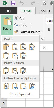
New Office, (2007, 2010, 2013) uses the Paste button in the ribbon to provide access (though there is still keyboard access with ALT+E+S).

Once you have something in the clipboard with the copy command, clicking the little arrow below Paste Icon in the ribbon gives you a lot more options. Each office application is slightly different  as to what you get.

Word has less options than Excel. Powerpoint and Outlook, Live Writer and Publisher etc. all use this feature differently. However each of them allow you to strip metadata (formatting etc.) from the actual text and just paste the text. This extremely useful when copying text from a web page, PDF file or some other heavily formatted document.

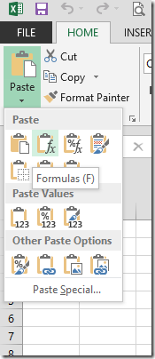
Hovering your mouse over any of the icons will give you a tool tip identifying it as per the example on the right.

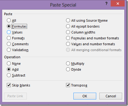
And clicking the Paste Special link at the bottom brings up the traditional dialog box.

Ill take you through the main ones for Excel.

• Paste Special Formulas Use this when you want to copy a formula but don't want to change the editing on the target cell(s)
• Paste Special Values Use this when you want to convert a selection (or single cell) from formulas or links to just the current calculated value. Full resolution of formulas to maximum decimal places will occur even if formatting doesn't show it. This is useful to cut links from external files, replace temporary formulas with actual results etc.
• Paste Special Links Use this to quickly paste the link to an external spreadsheet by copying from that sheet and paste links into the target cell(s)
• Paste Operation - Multiply, Add, Divide, Subtract These are very powerful tools. Try this:
  Find a selection of formulas (eg sums at the bottom of a range). Enter 0 (zero) in a blank cell then copy that cell.
  Select the range you want to alter and Paste Special Operation Multiply. (You may want to click Formulas as well so as to not change target cell(s) formatting).
  This will add to your existing formula *0 (and any required brackets) and the result will become zero. This can be used in all sorts of ways, - eg dividing numbers by 1,000 to change $ to $'000 etc.
• Paste Special Transpose Use this to alter the orientation of a selection of cells. Copy a column and turn it into a row and vice versa.

You can also combine options from each section as per the example below.

The IF function is a very useful logical tool. I have written an explanation on the IF Function before so I wont repeat that here. There are a number of other posts also that incorporate the use of the IF Function.

What I want to do is highlight a useful way to use the IF function.

I use it a lot to compare lists of data. today I had been sent some data in a spread sheet that contained email addresses. I had to create a mail out to those email addresses and when i did that I received a number of bounce backs for incorrect email addresses. I then received a second email from the original person containing a revised spread sheet with the corrections to email addresses. given that there were a large number of addresses and only a few changes I didn’t want to painstakingly work my way through the list looking for changes. Instead I copied the new list beside the old list and then wrote an if statement to compare the original with the revised. It is very simple and uses a 1 or 0 result. You could use anything there including TRUE or FALSE or “OK” and “ERROR” etc. Then a simple filter showed me the incorrect ones and the fixes i needed to apply in my mailing list.

Obviously I have obfuscated the email addresses in this example for privacy reasons.

The actual IF statement is very simple. In Cell C1 I wrote =IF(B2=A2,0,1). Filling it down is as simple as double-clicking the right hand bottom corner of the cell.

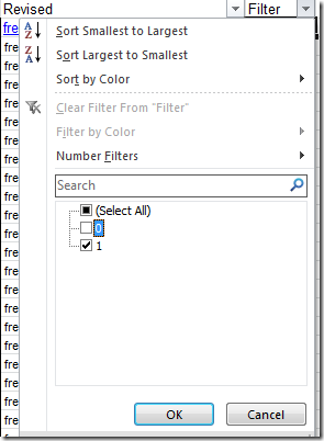
Then I added a simple filter to hide the correct results and only display those with differences.

I use this technique many times a week in comparing data lists.

While looking at previous posts to choose a different function for this weeks post I noticed that I have never written a post specifically about the most commonly used function in Excel, the SUM function.

So today’s post remedies that. Note this post is based on Excel 2010. Most of this is still relevant in Excel 2003 and Excel 2007 is largely the same as 2010. The main difference is the ribbon references in Excel 2007/2010 vs the toolbar in 2003.

First the Official Excel Help information.

Description

The SUM function adds all the numbers that you specify as arguments. Each argument can be a range, a cell reference, an array, a constant, a formula, or the result from another function. For example, SUM(A1:A5) adds all the numbers that are contained in cells A1 through A5. For another example, SUM(A1, A3, A5) adds the numbers that are contained in cells A1, A3, and A5.

Syntax

SUM(number1,[number2],...])
The SUM function syntax has the following arguments:
number1    Required. The first number argument that you want to add.
number2,,...    Optional. Number arguments 2 to 255 that you want to add.

Remarks

If an argument is an array or reference, only numbers in that array or reference are counted. Empty cells, logical values, or text in the array or reference are ignored.
If any arguments are error values, or if any arguments are text that cannot be translated into numbers, Excel displays an error.