Spy Journal 3.0 Filtering the web for you

I received this question on the website from Eric regarding conditional formatting:

Hi,

I have the same problem as a few people above but I don't think you got the point of the problem,

In xl2003 if you select A3:A9 and enter conditional format =B3 then select any other cell in the range it will show the conditional format for that cell e.g. A7 will show =B7

In xl2007 after following the same steps it will apply the correct formatting but if you select cell A7 to view the conditional format it will show as =B3. You get the same when checking any cell in range A3:A9.

This makes it near impossible to edit or amend or debug conditional formatting once entered.

Any advice would be appreciated.

Eric.

I started to post my answer and realised that i would be better off writing the whole thing as a blog post with some images to explain.

Hi Eric
i understand the problem and the first answer is that you cannot apply the same sort of logic between the two versions. The new versions (including 2010) manage conditional formatting completely differently, though some of the same concepts apply.
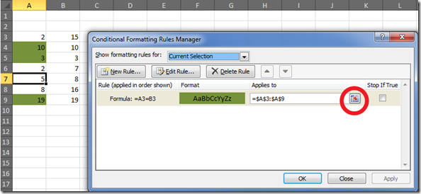
First of all your conditional format formula should be =A3=B3. This will apply the conditional format when the cell in A3 contains the same value as the cell in B3, and this will be relative - eg. when A7=B7 the cell in A7 will have the format applied. So you can see that the relative approach is correct in the conditional format manager in Excel 2007/2010
Second the problem you mentioned. When you look at the relative formula in cell B7 in excel 2003 it showed you just that formula. that is actually harder to debug if you think about it in Excel 2003 than in 2007/2010 as there is no way to see what other cells it also applies to. In Excel 2007/2010 the conditional format manager allows you to see the formula - and the range it is applied to and the little range box (circled in the image below) allows you to view this
The manager allows you to confine the selection to be evaluated to the selected cell(s), the current worksheet or other worksheets in the same workbook. If you then understand the relative / absolute nature of the formula you created then you can debug very successfully. I actually preferred this once I got a hang of using the manager to create sets of conditional formats than can be applied to multiple ranges simultaneously.

I had a reader request some help with Conditional Formatting in Excel 2007.

Hi

Baffled in trying to get to grips with conditional formating in 2007

Scenario :

Column A = Actual Result
Column B = Target
Column C = Needs to show
1) If Actual result is less than 90% of target turn font colour RED
2) If Actual result is >90% of target and is <100% of target turn font colour AMBER
3) If Actual result is >= 100% of target turn font colour GREEN

If column C meets criteria 1 use character "R", criteria 2 = "A" and criteria 3 = "G"

I can acheive 1 and 3 with =IF(a1b1,"G")) and then conditional format so that if contents of cell = R or G then colour font accordingly </B1,"R",IF(A1>

I`m stumped with the % factor and also think there might be a better way of doing it

Any help would be appreciated :)

Here is a solution to this problem.

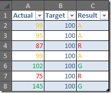
We formatted two columns to give two examples as to how it could be done.

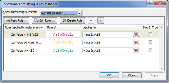
The actual column determines the percentage as part of the conditional format and formats in that way.

The result column formats on the “R”, “A”, and “G”.

The formula in Column C1 is =IF(A2/B2<1,IF(A2/B2<0.9,"R","A"),"G") and this can be copied down.

Here are the rules for Column A

There is just so much going on with the whole change over from Office 2007 to 2010, and for those of you still stuck in 2003, even more important for you to start convincing your organisations of the need to go straight to 2010.

We have been running the beta 2010 here solidly an all our main machines here for 2 months now, with some individual test machines previous to that. Unfortunately now we have to have test and development environments in both 2003 and 2007 so that has doubled our required number of Virtual Machines.

Following are some of the latest news and bits and pieces as well as some other MS Office related information I have come across recently.

Excel 2007 and 2010

Conditional formatting. Conditional formatting in 2007 is one of the main reasons people come to Spyjournal.biz. These two articles are the single most hit articles of the thousands here with over 50,000 views between them:

• Conditional formatting in Excel 2007 - entire row colours
• Excel 2007 Conditional Formatting

Amit Velingkar has written conditional formatting rules simplified while Dick Kusleika has written some code to list out all the conditional formatting rules in a worksheet

I have had a bunch of pretty cool Excel things to post up – and finally got around to clearing my flagged items and browser windows.

Conditional Formatting

I have written a couple of articles on Conditional formatting in Excel 2007 with lots of readers comments and requests for help. They are the two most read articles on this site.

• Conditional formatting in Excel 2007 - entire row colours
• Excel 2007 Conditional Formatting

I was very interested then to come across this article on Joseph’s site by Amit Velingkar where he shows you how to change the automatic colour ranges that are used in Excel 2007 for conditional formatting. He even includes some VBA code for this.