Spy Journal 3.0 Filtering the web for you

I had a reader request some help with Conditional Formatting in Excel 2007.

Hi

Baffled in trying to get to grips with conditional formating in 2007

Scenario :

Column A = Actual Result
Column B = Target
Column C = Needs to show
1) If Actual result is less than 90% of target turn font colour RED
2) If Actual result is >90% of target and is <100% of target turn font colour AMBER
3) If Actual result is >= 100% of target turn font colour GREEN

If column C meets criteria 1 use character "R", criteria 2 = "A" and criteria 3 = "G"

I can acheive 1 and 3 with =IF(a1b1,"G")) and then conditional format so that if contents of cell = R or G then colour font accordingly </B1,"R",IF(A1>

I`m stumped with the % factor and also think there might be a better way of doing it

Any help would be appreciated :)

Here is a solution to this problem.

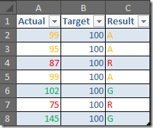
We formatted two columns to give two examples as to how it could be done.

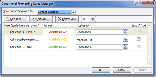
The actual column determines the percentage as part of the conditional format and formats in that way.

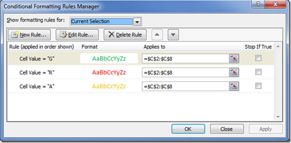
The result column formats on the “R”, “A”, and “G”.

The formula in Column C1 is =IF(A2/B2<1,IF(A2/B2<0.9,"R","A"),"G") and this can be copied down.

Here are the rules for Column A

And here are the rules for Column C

Thanks to Nick who works for me for developing this solution for me.