Spy Journal 3.0 Filtering the web for you

Data Filters are a very powerful way of analysing tables of data in Excel. Put simply they are a way of reducing the table down to just the items you want to see based on the selections you choose.

For example a simple table like this one, may have several hundred or thousand rows of data. However there may be only a few lines you are interested in. For example you may be only interested in people under the age of 18 or sales amounts that are negative (indicating a refund) or only see sales of red Ferraris.

Turning on the Filters

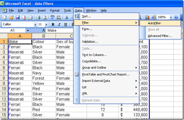
In Office 2003 Turn on the filters by selecting any cell in your table (contiguous section of data) and selecting Data, Filter, Auto Filter from the menu. (Keystroke ALT D F F)

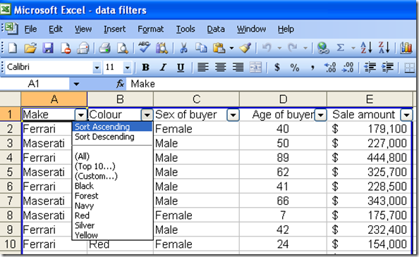
The arrows will show up as in the next picture.

In Office 2007 the filters are quite different. They are turned on differently and behave differently also.

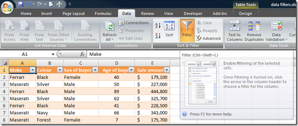
Turn them on by selecting  any cell in the data table and clicking Data, then Filter. (Keystroke CTRL+SHIFT+L)

Turning off the filters in both versions is simply repeating the same clicks or keystrokes.

Filtering the data

Once you have the filters turned on you are able to reduce the visible cells by clicking the arrow for any column and then selecting from the available items.

In 2003 this looks like this:

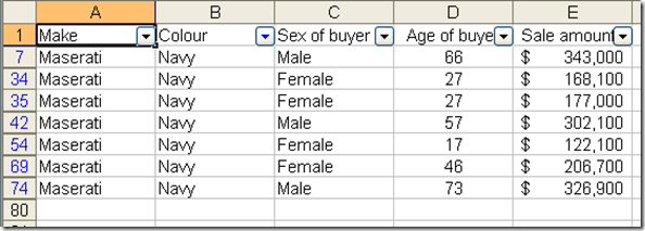
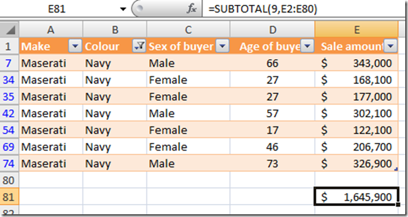
Selecting Navy reduces the data set from, in this case, 79 items to 7. Note the blue row numbers. These indicate the filtering that has hidden the rows between. Some formulas only work with visible cells. And these hidden cells will now be excluded from those formulas.

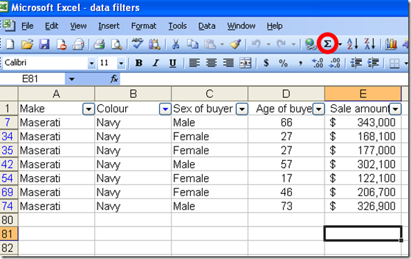
SUBTOTAL for example is a formula that will sum only visible cells. Select the cell two cells below the bottom of the table under a value column (Sales) and then double click the SIGMA Sum icon on the toolbar.

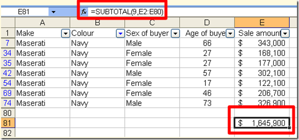
Note how the resulting formula displays only the value of the visible cells, though it is evaluating all cells in the column of the table.

The same effect can be achieved in Office 2007. However the selection process is somewhat different.

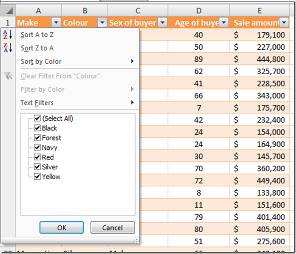
When you select the arrow you are presented with a number of different options. The sort function is made available from this menu. The custom number and text filters are contextual and made available through a right arrow and secondary menu.

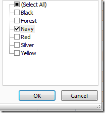
The filters based on the actual data in the column are now presented as check boxes with the default being they are all selected. You can turn off all the items you don’t want to see, or in this case you can turn off Select All and then turn on Navy.

Now Click OK and the resulting data set will display the same items – those sales where the car colour was Navy.

Unfortunately in Office 2007 double clicking the sigma function button won’t give you subtotals but just the normal SUM formula. However entering the SUBTOTAL formula in will get the same mathematical result as Excel 2003.

There is a lot more that can be done with filters. Next time we will look at using the custom text and number filters.

See my previous posts on this subject and similar subjects.

Office 2007 Excel Data Auto Filter

Using the Advanced Filter in Excel

Turning Excel Auto Filters on and off in VBA

Creating Subtotals in Excel

Using the Advanced Filter Function in Excel to locate unique records

Saving Autofilter Criteria