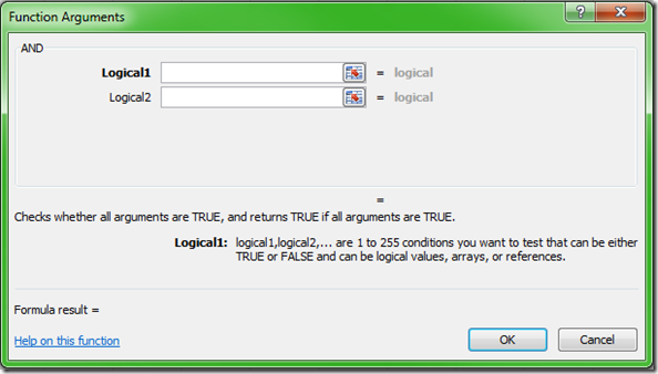
AND
Excel function of the week - AND
Thu, 23/12/2010 - 9:28am — jethroThe AND function takes each of the conditions inside the brackets and evaluates for their truth, and then multiplies the results together. TRUE = 1 and FALSE = 0. So if any condition is FALSE then the overall statement returns FALSE.
The formula for AND needs to be placed in brackets with each of the conditions separated by a comma. For example =AND(H1<1,G1>1)
In this instance the function will evaluate H1 to see if the value is less than 1. if it is then it will return TRUE or 1 and if not FALSE or 0. Then it will do the same for G1.
The two values are multiplied together and the answer is then either 1 or 0, TRUE or FALSE.
The Excel Help says:
One common use for the AND function is to expand the usefulness of other functions that perform logical tests. For example, the IF function performs a logical test and then returns one value if the test evaluates to TRUE and another value if the test evaluates to FALSE. By using the AND function as the logical_test argument of the IF function, you can test many different conditions instead of just one.
Conditional formatting in Excel 2007 - entire row colours
Fri, 19/09/2008 - 11:03am — jethroI had an interesting question about conditional formatting posed in the comments by Stephen.
In a new sheet, I am trying to make a whole row turn red, green or amber depending on the value of one cell in that row, so I can easily see which jobs we have won, lost or are pending. Any 'IF' conditional formula I write gets thrown out by Excel. What am I doing wrong?
I promised him an answer so here it is.
For this exercise I am making some assumptions.
- You are using Excel 2007 format Excel spreadsheet (.xlsx or .xlsm). These instructions will not work in detail for Excel 2003, though the concept is similar.
- That there are 3 conditions we are looking for. Of course Excel 2007 allows more than 3 conditions so you can add more if you need. (One of the improvements on Excel 2003 that only allowed 3 rules)
- That the entire row is needed to be coloured. If you need a smaller section than change the formulas accordingly.
- That the entire worksheet needs this formatting. If you need a smaller section than change the formulas accordingly.
- That the conditional formats are going to be based on a cell that returns a specific result based on some other rule.


Recent comments
10 years 37 weeks ago
10 years 37 weeks ago
10 years 39 weeks ago
10 years 39 weeks ago
10 years 39 weeks ago
10 years 39 weeks ago
10 years 39 weeks ago
10 years 39 weeks ago
10 years 39 weeks ago
10 years 39 weeks ago