IF
Excel Tools and News from the web
Fri, 01/05/2009 - 11:01am — jethroI have had a bunch of pretty cool Excel things to post up – and finally got around to clearing my flagged items and browser windows.
Conditional Formatting
 I have written a couple of articles on Conditional formatting in Excel 2007 with lots of readers comments and requests for help. They are the two most read articles on this site.
I was very interested then to come across this article on Joseph’s site by Amit Velingkar where he shows you how to change the automatic colour ranges that are used in Excel 2007 for conditional formatting. He even includes some VBA code for this.
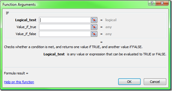
Excel Function of the Week - IF
Mon, 20/10/2008 - 7:24pm — jethroI have decided to write a short post once a week looking at a single Excel function. This week we are going to look at the IF function.
Definition from Excel Help
The IF function returns one value if a condition you specify evaluates to TRUE, and another value if that condition evaluates to FALSE. For example, the formula =IF(A1>10,"Over 10","10 or less") returns "Over 10" if A1 is greater than 10, and "10 or less" if A1 is less than or equal to 10.
Syntax
IF(logical_test, value_if_true, [value_if_false])
My explanation
The IF function is best thought of as a solution to “either - or” scenarios. Here are some good examples with the syntax to use for each one.
Developing in Excel 2007
Wed, 15/10/2008 - 12:00pm — jethroI much prefer working in Excel 2007 to Excel 2003. Despite the issues with backward compatibility, there are a lot of advantages and benefits to using the new version.
Some little things that have been changed are
The previous limit on nested brackets in formulas from 7 has been increased to 64. I used this today
The number of columns and rows has increased. I used this today.
I had to develop a file for a client that involved a complex work roster arrangement to calculate days off in repeating 2, 3 or 4 week cycles for the next 20 years.
Here is the nested formula that got me the logic for a roster.
=IF($X5>=AJ$4,$X$4,IF($Y5>=AJ$4,$Y$4,IF($Z5>=AJ$4,$Z$4,IF($AA5>=AJ$4,$AA$4,IF($AB5>=AJ$4,$AB$4, IF($AC5>=AJ$4,$AC$4,IF($AD5>=AJ$4,$AD$4,IF($AE5>=AJ$4,$AE$4,IF($AF5>=AJ$4,$AF$4,$AG$4)))))))))
I then used one formula to generate over 600,000 cells and create a map that looks like this.
Finding MAX date with an Array Formula in Excel
Tue, 09/10/2007 - 8:15am — jethroLast week I was struggling with getting an array formula to work properly with the MAX function.
I had a column of business units, a column of dates and a status column.
I wanted to find the most recent date for any given business unit where the status was a particular criteria.
I did try using Bob Phillip's sum product page and Chris Pearson's array formulas page, but it still wasn't working right. Fortunately Bob emailed me with the answer and explained it very well. (I was missing the IF function).
Heres the formula and what Bob said about it:
=MAX(IF((criteria_range1="criteria1")* (criteria_range2="criteria2")* (criteria_range3="criteria3"), date_range))


Recent comments
10 years 37 weeks ago
10 years 37 weeks ago
10 years 39 weeks ago
10 years 39 weeks ago
10 years 39 weeks ago
10 years 39 weeks ago
10 years 39 weeks ago
10 years 39 weeks ago
10 years 39 weeks ago
10 years 39 weeks ago