Spy Journal 3.0 Filtering the web for you

The named range feature in Excel has been there for a long time. However the interface for the Name Manager changed in Excel 2007 and Excel 2010.

This article explains how to use the new name manager.

Firs of all let me explain what the Name Manger is and what it does.

From the Excel Help:

A name is a meaningful shorthand that makes it easier to understand the purpose of a cell reference, constant, formula or table. each of which may be difficult to comprehend at first glance. The following information shows common examples of names and how they can improve clarity and understanding.

I use Range Names to clearly define parts of the spreadsheet data tables and lists that i want to refer to in formulas with a easily understood name rather than the actual sheet and cell reference. This makes it much easier to audit a spreadsheet for accuracy.

To open the Name Manager dialog box, on the Formulas tab, in the Defined Names group, click Name Manager. There is a keyboard short cut of CTRL + F3.

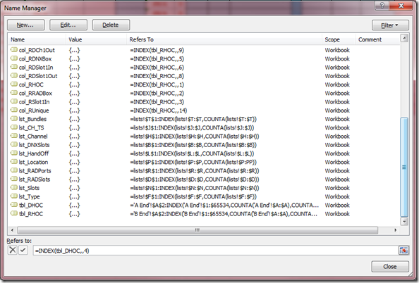
Here is one from a spread sheet tool I am working on.

In this case most of the named ranges are using the Index function in order to be a dynamically expanding range. (see previous articles and links to using INDEX to create dynamic range names)

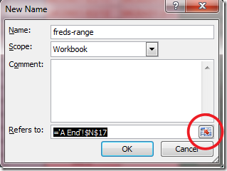
Adding a new range is very simple, click New and type the range name and then use the range selector to go and select the range. But there are some shortcuts.

You will note from my example above that there is a very structured range name convention that I am using.

I use a prefix to define the range types as follows:

• rng_ for a single cell range
• lst_ for a list – usually a vertical column that needs to expand as new items are added to it. I use this for dropdown lists.
• tbl_ for a multi column and row table – usually for a lookup table that returns results used to search a data table
• data_ for a large data table that needs to be used in the spreadsheet – eg raw data.
• col_ for a column in a data range
• row_ for a row in a data range

The next thing I do is consider what my convention will be. In this case i have several defined sheets with similar information each of which is an In or Out. So the convention identifies the type of sheet, the data type and the In or Out nature of the data. building a convention like this and documenting it allows yourself and any other developers to easily understand from the names used in a formula what data is being accessed.

E.g. here is a formula from this file. =INDEX(col_RDSlot1Out,MATCH($W2,col_RUnique,0))&"/"&INDEX(col_RDCh1Out,MATCH($W2,col_RUnique,0)). I can look at this and understand it almost instantly.

The next thing i do after working out my convention is to work out all the range names i will need. I then type them in cells. This can be done quickly by copying and pasting or filling down and editing as required.

The reason for doing this is because Excel is very smart – if you select any of these cells and open the Name Manager and hit New (CTRL+F3, ALT+N) it will prefill the range name with the text from the cell. This can make it much faster to create a large number of range names. In addition if you are using a standard formula with just minor changes for consecutive ranges then you can copy and paste the same formula into the range name and then just edit it. Note you cannot use the left and right arrow keys while editing the range name.

I hope these hints will assist you in using the Name Manager more efficiently.

I had a colleague ask me this question today. (edited to protect the innocent – you know who you are!)

I copy data out of E_____ (am sure you have heard of it), and paste it into an excel spreadsheet.  I have a couple of pivot tables hanging off the back of this data.  As this is project data, the longer the project goes on, the larger the dataset gets.  Is there any way in VBA that I can get the pivot table to auto-expand the data set that it is using? 

Here is my answer.

Hey W__

There is a simple solution that doesn’t require any vba at all

First you will need to make a dynamic range name that covers the data being pasted.