Spy Journal 3.0 Filtering the web for you

This is a “real” blog post. Doesn’t feel that way yet? That’s cos I am still rambling. Or is that why it is a real blog post? Maybe this has something to do with the fact that it is the absolutely unheard hour of 6:30am and I was awake at 5:30 and have consumed a very nice coffee and am buzzing!

So lets deal with the facts involved here. First off the screen door slamming about 3 metres from head while I was asleep and in the middle of a strange confused dream where I was involved in counter terrorist warfare including a shootout in a barn where I stopped bullets matrix slow motion style using a leather cushion and then encourage the last remaining terrorist to shoot himself so I could rescue the civilian hostage (predictably a woman) rudely awoke me. Particularly as that was followed up with scratching sounds on the door. I went to the door with my big stick (kept beside my bed) and found a gecko on the inside: conclusion neighbours cat (that I daydream about sending to cat heaven) was chasing the gecko and leaped at the door slamming it shut.

When I wrote the how to use VLOOKUP and HLOOKUP article a few weeks ago I hinted at writing how to use the COLUMN, ROW, MATCH, INDEX and OFFSET functions to enhance the use of the VLOOKUP and HLOOKUP functions. Today we will look at the use of MATCH.

First of all here is a common scenario.

You create a table of say 4 columns, and then in another sheet you create a VLOOKUP function that returns results from the 4th column. EG =VLOOKUP(lookup_value,table_range,4,FALSE) where the 4 relates to the 4th column. This works great until one day you (or your colleagues) delete the 3rd column in the table, or insert another column in the middle of the table. Now your VLOOKUP fails as the 4th column either doesn’t exist, or is now actually the 5th column. In this case the VLOOKUP formula you created is just not flexible enough to handle the changes.

The following explanation builds on the dynamic range name process defined in my article written back in 2004. You will need to create a dynamic range name (in this example called table_header) that works on the header row of the table you are performing the VLOOKUP on.

In Excel 2007 Use the Name Manager from the Formula tab. In Excel 2003 and earlier use Edit Insert Name Define. In both versions CTRL F3 is the keyboard short cut.

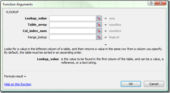
I realised that when I wrote the ISNA function article that I had never written an explanation of VLOOKUP. I want to write up explanations for a umber of other functions in the future like COLUMN, ROW, MATCH and INDEX followed by OFFSET. All these make lots of sense when you use them with the VLOOKUP function. So I though it best to start with this function. I will also say that everything I write about VLOOKUP here applies to HLOOKUP as well. the only difference is the orientation, that is VLOOKUP looks across columns from left to right, and HLOOKUP looks down rows from top to bottom.

The built in Excel Help is very good at helping with this function. However it doesn't point out many of the pitfalls than occur in common use.

The ISNA function is an Information Function. It is is used to return information about the status of a cell, or specifically another functions results. The most common use I have for this function is to validate the VLOOKUP function. If the VLOOKUP function is looking for a value that can not be found in the lookup range, then it will return #N/A as the result. Thus it is good to wrap that function in an IF Statement using the ISNA function to replace the #N/A results with something else – e.g. a text string such as “error” or maybe a zero.

=IF(ISNA(VLOOKUP(A1,$B:$B,1,FALSE))=TRUE,"error",VLOOKUP(A1,$B:$B,1,FALSE))

Remember the ISNA function returns a TRUE or FALSE. These equate to a 1 or 0 so can be used in formulas such as array formulas as well.